Parallel Training
InternEvo supports tensor parallel, pipeline parallel, sequence parallel, data parallel, and ZeRO1.5 to parallelize the training pipeline. When initializing the distributed environment, we need to specify tensor parallel size, pipeline parallel size, data parallel size, and ZeRO1.5 strategy.
The parallel setting of InternEvo is fully config-driven, and you can change the parallelism by modifying config file. An exmaple parallel training configuration can be defined as follows:
parallel = dict(
    zero1=dict(size=8),
    tensor=dict(size=1, mode="mtp"),
    pipeline=dict(size=1, interleaved_overlap=True),
    weight=dict(size=1, overlap=True, memory_pool=True),
)
zero1: zero parallel strategy, divided into the following three cases, the default value is -1
When
size <= 0, the size of the zero1 process group is equal to the size of the data parallel process group, so the optimizer state parameters will be split within the data parallel range.When
size == 1, zero1 is not used, and all data parallel groups retain the complete optimizer state parameters.当
size > 1且zero1 <= data_parallel_size,则 zero1 进程组是数据并行进程组的子集
tensor: tensor parallel strategy
size: int, tensor parallel size, usually the number of GPUs per node, the default value is 1
mode: the tensor parallel mode, should be in [‘mtp’, ‘msp’, ‘fsp’, ‘isp’],
mtp: defaults to ‘mtp’, means the pure megatron tensor parallel without sequence parallel
msp: megatron tensor parallel with sequence parallel, sequence parallel size = tensor parallel size
fsp: tensor parallel by flash-attn with sequence parallel, sequence parallel size = tensor parallel size
isp: customed intern sequence parallel without tensor parallel, can be used with weight parallel
pipeline: pipeline parallel strategy
size: pipeline parallel size, the default value is 1
interleaved_overlap: bool type, when interleaved scheduling, enable or disable communication optimization, the default value is False
weight: weight parallel strategy, only can be used with ‘isp’ tensor parallel mode
size: weight parallel size, the default value is 1
overlap: bool, enable/disable all_gather/reduce_scatter communication overlap, defaults to False
memory_pool: bool, enable/disable memory pool, defaults to False
Note: Data parallel size = Total number of GPUs / Pipeline parallel size / Tensor parallel size
Tensor Parallel
The InternEvo system version v0.3.0 has significant updates in the tensor parallelism strategy. The current tensor parallelism supports four modes: [‘mtp’, ‘msp’, ‘fsp’, ‘isp’]. The first three modes are based on the Megatron-LM’s tensor parallelism and sequence parallelism strategy. The last mode is a self-developed strategy by the InternEvo system, which is a new sequence parallelism method that can be used in conjunction with weight parallelism. The following provides a detailed explanation of the differences among these tensor parallelism modes.
MTP
MTP (Megatron-LM Tensor Parallel) is the default tensor parallelism model, inspired by the Megatron-LM Tensor Parallel parallel scheme, as referenced in the paper Megatron-LM Tensor Parallel. The following diagram illustrates the Transformer layer with tensor parallelism:
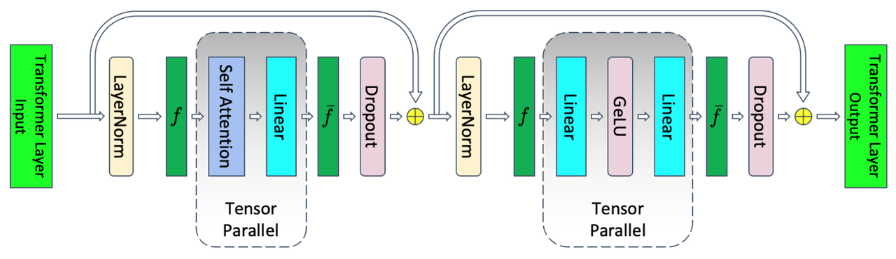
Transformer layer with tensor parallelism.
MTP primarily applies tensor parallelism operations to the attention and the linear module. Assuming the tensor parallelism size is tp, the sequence length of input data is seqlen, and the hidden layer size is hidden size, then the shape of the activation values generated during tensor parallelism is [seqlen, hidden_size/tp].
The communication introduced by MTP is illustrated in the above diagram, where f and f̄ are conjugates. In the forward pass, f corresponds to a no-operation, while in the backward pass, it involves an all-reduce operation. On the other hand, f̄ performs an all-reduce operation in the forward pass and is a no-operation in the backward pass.
MSP
MSP (Megatron-LM Sequence Parallel) is adopted from the Megatron-LM Sequence Parallel parallel scheme. The following diagram illustrates the Transformer layer with both tensor parallelism and sequence parallelism:
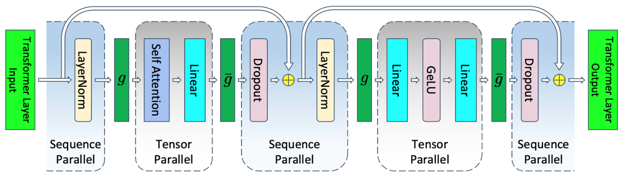
Transformer layer with tensor and sequence parallelism.
Compared to MTP, it is evident that MSP primarily focuses on modules without tensor parallelism, such as LayerNorm and Dropout, and performs sequence parallelism operations. It is important to note that the size of sequence parallelism is equal to the size of tensor parallelism, and they share the same communication group. Assuming the tensor parallelism size is tp, the input data has a sequence length of seqlen, and the hidden layer size is hidden size, the shape of activation values during sequence parallelism is [seqlen/tp, hidden_size], while during tensor parallelism, it is [seqlen, hidden_size/tp].
In comparison to MTP, there are variations in the communication primitives in MSP, as illustrated in the diagram above, where g and ḡ are conjugates. In the forward pass, g performs an all-gather operation, while in the backward pass, it undergoes a reduce-scatter operation. On the other hand, ḡ conducts a reduce-scatter operation in the forward pass and an all-gather operation in the backward pass.
In the forward pass, the communication of g occurs at the junction of sequence parallelism and tensor parallelism, performing an all-gather operation along the seqlen dimension of activation values. After this communication is completed, the shape of the activation values becomes the full [seqlen, hidden_size], and then it enters the scope of the tensor parallelism module. The communication of ḡ is situated at the junction of tensor parallelism and sequence parallelism, requiring the transformation of the all-reduce communication operation from MTP into a reduce-scatter operation to achieve the split along the seqlen dimension. This results in the activation values having a shape of [seqlen/tp, hidden_size], enabling a smooth transition into the sequence parallelism phase. The same principles apply during the backward pass.
FSP
FSP (Flash-Attn Sequence Parallel) is a sequence parallelism implementation inspired by the flash attention scheme, as referenced in flash attention. The only difference between this implementation and MSP is that, after the g performs all-gather communication, MSP stores a complete copy of the input data for backward computation, while FSP only retains the input data split into seqlen segments. Therefore, during backward computation, an additional all-gather operation is needed to retrieve the complete input data.
Therefore, in terms of performance comparison between FSP and MSP, FSP tends to have a smaller memory footprint. However, the introduction of additional all-gather communication can lead to a reduction in the training speed, denoted as TGS.
ISP
ISP (Intern Sequence Parallel) is a flexible and scalable sequence parallelism solution developed in-house by the InternEvo system. It supports the decoupling of tensor parallelism and sequence parallelism, enhancing training performance through the overlap of computation and communication. Additionally, it incorporates memory pool management to reduce the likelihood of memory fragmentation, thereby improving memory utilization.
Taking the configuration file configs/7B_isp_sft.py as an example, set the tensor.mode field to isp, where the tensor.size field represents the size of data split along the seqlen dimension. The ISP algorithm can be combined with weight parallel, where the weight.size field represents the model weight split size. Setting weight.overlap to True enables computation and communication overlap, enhancing training performance. Setting weight.memory_pool to True activates the memory pool management feature, which helps to some extent in reducing the likelihood of GPU memory fragmentation and improving memory utilization.
parallel = dict(
    zero1=dict(size=-1),
    tensor=dict(size=2, mode="isp"),
    pipeline=dict(size=1, interleaved_overlap=True),
    weight=dict(size=4, overlap=True, memory_pool=True),
)
As illustrated in the diagram below, there is a Transformer layer with both sequence parallelism and weight parallelism:

As shown in the figure, the sequence parallelism scope of ISP covers the entire Transformer model layer, while the weight parallelism primarily targets the Linear module within the Attention and MLP Block.
The changes in communication primitives are as follows: during the forward pass, each Linear module requires all-gather communication for model weight. In the backward pass, before performing the backward computation, each Linear module requires all-gather communication for model weight. After the backward computation, there is a reduce-scatter communication operation for the gradients of model weights.
It is important to note that, in comparison to MSP and FSP, there are some changes in communication primitives for attention score calculation in ISP. For instance, before and after Self-Atten, an additional all-to-all communication operation is introduced to transpose the shape of activation values. The purpose is to maintain the original tensor parallelism pattern during the attention score calculation.
For more design details and performance evaluation of the ISP algorithm, please refer to the paper InternEvo: Efficient Long-sequence Large Language Model Training via Hybrid Parallelism and Redundant Sharding.
Pipeline Parallel
InternEvo uses 1F1B (one forward pass followed by one backward pass) for pipeline parallel. For 1F1B strategy, there are two implementations:
non-interleaved scheduler, which is memory-efficient
interleaved scheduler, which is both memory-efficient and time-efficient.
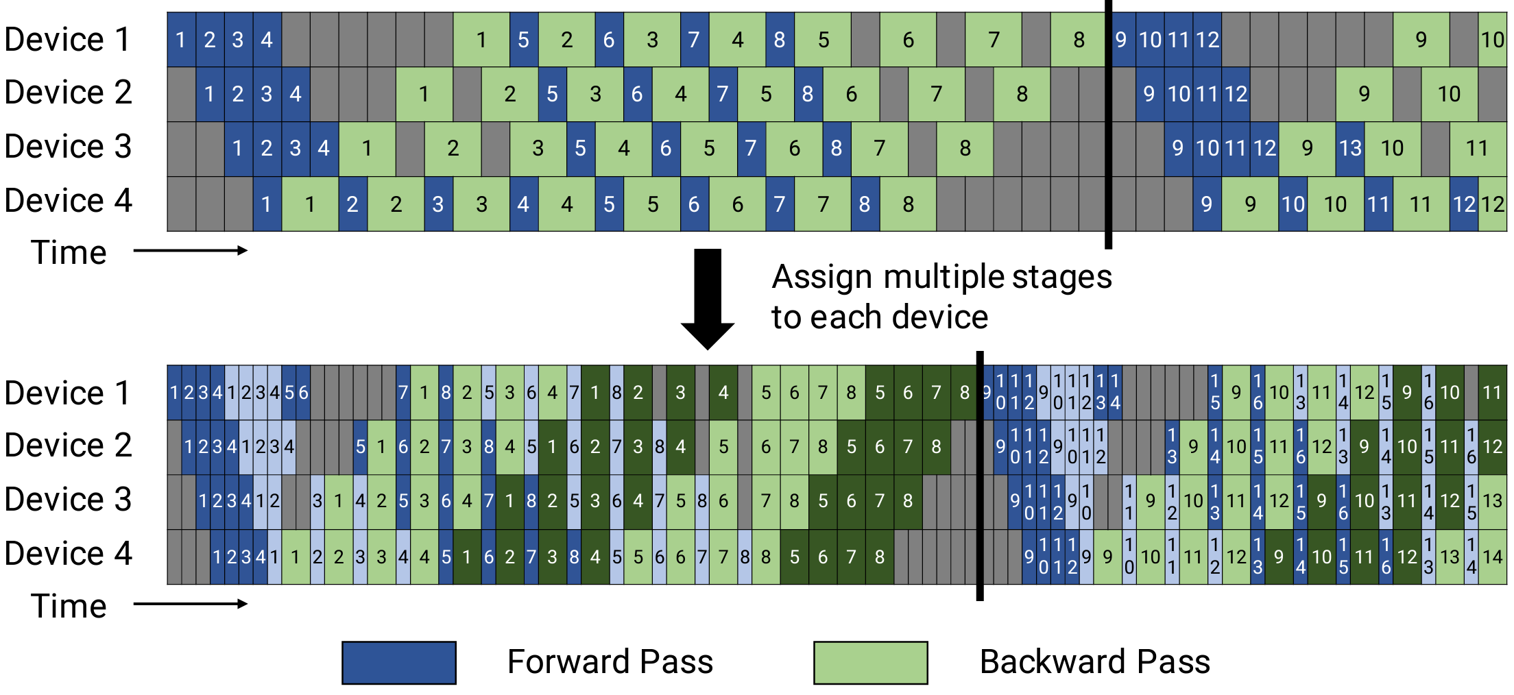
Non-interleaved and interleaved scheduler for 1F1B pipeline parallelism, adopted from Megatron-LM
scheduler for non-interleaved 1F1B strategy
To use non-interleaved pipeline scheduler, users need to set model.num_chunks = 1 in the config file.
scheduler for interleaved 1F1B strategy
To use interleaved pipeline scheduler, users need to set model.num_chunks > 1 in the config file.
Asynchronous communication will be enabled in 1F1B stage to make full use of uplink/downlink bandwidth and achieve communication overlap.
When parallel.pipeline.interleaved_overlap = True, function InterleavedPipelineScheduler._run_1f1b_loop_with_overlap will be called and internlm.core.communication.AsynCommunicator will be created for managing async communication.
The difference between 1F1B stage without overlap and 1F1B stage with overlap is shown as follows:
# The 1F1B stage without overlap consists of the following steps:
1. Perform the forward pass.
2. Perform the backward pass.
3. Send the forward output of this iteration to the next stage, and send the backward output of this iteration to the previous stage, and receive the forward and backward inputs for the next iteration.
# The 1F1B stage with overlap consists of the following steps:
1. Perform the forward pass.
2. Check if the backward input is ready.
3. Send the forward output and receive the forward input for the next iteration.
4. Perform the backward pass.
5. Check if the forward input is ready.
6. Send the backward output and receive the backward input for the next iteration.
Data Parallel
InternEvo supports data parallel. For data parallel:
Data parallel size = Total number of GPUs / Pipeline parallel size / Tensor parallel size
ZeRO1.5
The implementation of ZeRO1.5 uses the concept of hierarchical sharding via config value parallel.zero1, which enables sharding within local nodes.
If
parallel.zero1 <= 0, the size of the zero process group is equal to the size of the dp process group, so parameters will be divided within the range of dp.If
parallel.zero1 == 1, zero is not used, and all dp groups retain the full amount of model parameters.If
parallel.zero1 > 1andparallel.zero1 <= dp world size, the world size of zero is a subset of dp world size. For smaller models, it is usually a better choice to split the parameters within nodes with a settingparallel.zero1 <= 8.
Furthermore, you can enable communication-computation overlap, set bucket reduce size, gradient clipping parameters in the config file.
hybrid_zero_optimizer = dict(
    # Enable low_level_optimzer overlap_communication
    overlap_sync_grad=True,
    overlap_sync_param=True,
    # bucket size for nccl communication params
    reduce_bucket_size=512 * 1024 * 1024,
    # grad clipping
    clip_grad_norm=1.0,
)
There are two communication optimizations worth paying attention to here:
overlap_sync_grad: If set True, overlapping training backward pass with gradients’ all-reduce communication.
overlap_sync_param: If set True, overlapping parameters’ broadcast communication with next step’s forward pass.
These optimizations can speed up the training process and improve training efficiency.